Every investor who plans a twin-screw extruder plastic compound factory eventually asks the same practical question: how many months will it take before the plant pays back the money tied up in the line? The answer is rarely a single number. A co-rotating parallel twin-screw compounding line is a capital-intensive asset, and its recovery speed depends on throughput, utilization, yield, gross margin, shift organization, and how quickly the plant climbs to full capacity. This article builds a transparent payback model expressed entirely in months, percentages, and an indexed baseline of 100 points, so you can compare configurations without quoting any currency. Whether you run a PP filled masterbatch line, a glass-fiber reinforced engineering compound, a halogen-free flame-retardant grade, a color masterbatch, or a TPE/TPV specialty, the recovery logic is the same and the levers are repeatable.
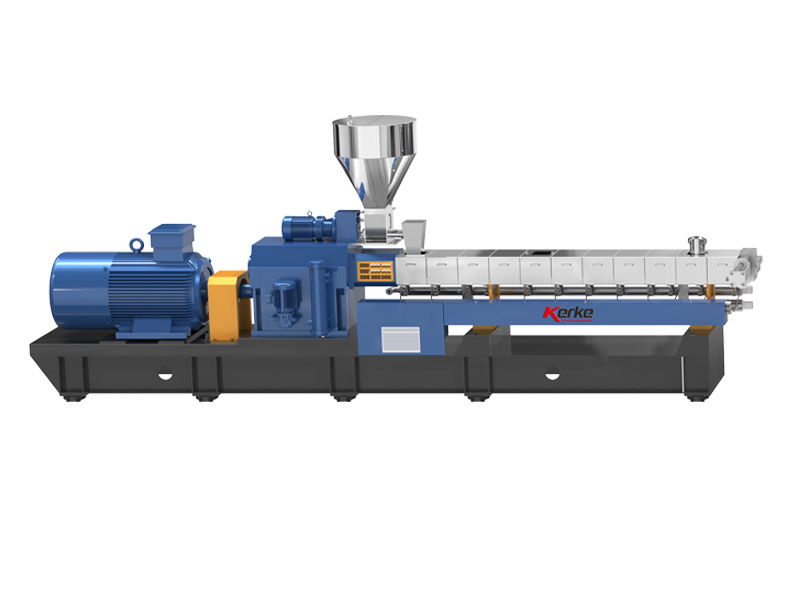
Kerke, a Wanplas factory, has supplied parallel co-rotating twin-screw compounding extruders such as the KTE series for more than 12 years, with 2,000-plus machines running in 70-plus countries. We write this guide from that field experience. The Wanplas brand as a whole covers the full plastic machinery chain, but here we focus strictly on the payback cycle of a compounding plant rather than a full cost ledger. A companion article on the same site breaks down the complete operating cost detail; this piece keeps its attention on the recovery model, the sensitivity of each variable, and the concrete actions that compress the payback window.
Why Payback in Months Matters More Than Headline Price
The sticker price of a twin-screw extruder is the least useful number when you evaluate a project. Two lines with the same headline investment can return capital in 22 months or 46 months depending on how they are run. Decision makers in compounding should treat the payback cycle as the primary ranking metric because it captures both the equipment and the business model around it. A shorter payback reduces exposure to demand swings, raw material price shifts along the resin chain, and competitive entry. It also frees cash for the next capacity step sooner.
We deliberately avoid currency units in this model. Currency rates, freight, and local labor rates vary widely across regions, and quoting them would date the analysis. Instead we anchor everything to a baseline configuration set at 100 index points and to ratios and percentages that hold true regardless of local economics. The months figure you read here is a structural result of utilization, margin, and yield, not a currency forecast. That is exactly what makes the model portable from a greenfield plant in one continent to a capacity expansion in another.
The payback cycle in months is the single most decision-relevant metric for a compounding line because it merges equipment choice, product mix, and operating discipline into one comparable number.
The Payback Model: Static and Dynamic Recovery
The recovery model starts from a simple ratio. The static payback period in months equals the initial investment index divided by the monthly net cash flow index. We set the baseline configuration at 100 index points, so a line that costs twice the baseline carries an investment index of 200, and a line half the baseline carries 50. The monthly net cash flow index reflects contribution after direct operating cost but before depreciation and financing, expressed on the same index scale.
Static payback months = Initial investment index divided by Monthly net cash flow index. If the baseline line carries an investment index of 100 and generates a monthly net cash flow index of roughly 3.3, the static recovery lands near 30 months. That single ratio is the backbone of every table in this article. The advantage of the index method is that you can scale any configuration by multiplying the investment index and adjusting the cash flow index for utilization, margin, and yield, then re-dividing.
Dynamic payback adds the time value of money. Each monthly cash flow is discounted by a monthly rate derived from the annual cost of capital. Typical project discount rates for a compounding expansion run from 8 percent to 12 percent per year, which translates to a monthly rate near 0.65 percent to 0.95 percent. The dynamic payback is the smallest number of months at which the sum of discounted cash flows reaches the investment index. Compared with the static method, a 10 percent annual discount rate typically extends recovery by 2 to 4 months on a 24 to 36 month baseline. The sensitivity of that extension is itself worth modeling before you commit capital.
The model also needs a ramp-up correction. No compounding plant reaches nameplate on day one. Realistic ramp-up runs 3 to 9 months, and during that window utilization sits at 40 to 70 percent of nameplate. Because cash is generated only on sold good product, the effective payback clock starts when contribution begins, not at commissioning. We therefore treat ramp-up as a multiplier on the early cash flow and a direct add-on to the recovery period. A plant that ramps in 4 months rather than 8 months can pull its effective payback forward by a full quarter.
Investment Composition Indexed Against a 100-Point Baseline
Before computing months, you must understand where the investment index comes from. The table below decomposes a baseline production-scale twin-screw compounding line into its constituent shares, with the whole set to 100 index points. This view helps you see which upgrades move the index most and therefore which choices most affect the denominator of the payback ratio.
Investment composition indexed to a 100-point baseline
| Investment component | Index share (baseline = 100) | What it covers |
|---|---|---|
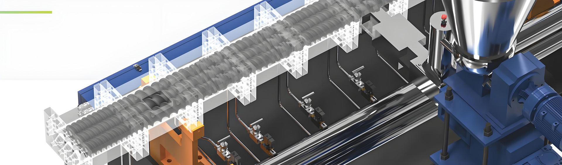
| Main extruder (twin-screw, gearbox, motor) | 38 | Barrel, co-rotating screws, high-torque gearbox, main drive, control cabinet |
| Auxiliary line (feeding to packing) | 22 | Loss-in-weight feeder, side feeder, screen changer, die, pelletizing, vibrating screen, packing |
| Building and power distribution | 14 | Workshop preparation, transformer, cable, compressed air, civil works |
| Central feeding system | 8 | Silos, vacuum conveying, dosing buffers for multi-material plants |
| Cooling water and chiller | 7 | Cooling tower, chiller, pump loop, temperature control |
| Dust and environmental control | 5 | Dust collection at feeders, odor and fume treatment |
| Laboratory and testing | 4 | Melt flow rate tester, injection sample molding machine, universal tester, glow-wire and vertical burn |
| Working capital buffer | 2 | Spare screw elements, screen packs, initial raw material inventory |
The main extruder and the auxiliary line together account for 60 index points. That is why screw diameter, L/D ratio, and pelletizing method dominate the investment index. A longer barrel or an underwater pelletizing system adds points here. The building, power, and cooling shares are comparatively fixed once you choose a site, so they do not scale strongly with screw diameter. The laboratory share looks small at 4 points but it is decisive for yield, because in-line melt flow rate checks and mechanical property verification prevent off-spec shipments that would otherwise destroy margin.
Typical Compounding Line Configurations and Capacity Tiers
Co-rotating parallel twin-screw extruders for compounding span a clear ladder of screw diameters and throughput. The table maps each diameter band to its typical throughput, the configuration around it, the product families it suits, and the resulting investment index relative to the 100-point baseline. Throughput ranges reflect continuous operation at good utilization, not peak test runs.
Capacity tier, configuration, product fit, and investment index
| Screw diameter | Throughput (kg/h) | Typical configuration | Best-fit products | Investment index |
|---|---|---|---|---|
| Phi 35 | 200 to 350 | Lab or pilot, single loss-in-weight feeder, strand pelletizing | Color masterbatch trials, additive masterbatch, R&D | 35 to 50 |
| Phi 50 | 500 to 800 | Pilot production, one side feeder, water-ring pelletizing | Small-batch color, TPE, specialty compounds | 60 to 75 |
| Phi 65 | 800 to 1200 | Production, loss-in-weight + side feeder, vacuum vent, water-ring or strand | Filled masterbatch, CaCO3 fill, GF compounds, FR grades | 95 to 110 (baseline 100) |
| Phi 75 | 1200 to 1800 | Production, twin side feeder option, continuous screen changer | High-volume masterbatch, GF-PA, halogen-free FR | 120 to 150 |
| Phi 95 | 2000 to 3000 | Heavy production, multiple side feeders, underwater pelletizing, central feeding | Commodity-filled volume, large GF lines, cable compounding | 170 to 230 |
Notice that moving from Phi 65 to Phi 95 more than doubles the investment index while throughput rises roughly 2.5 times. That ratio is favorable only if utilization stays high. A Phi 95 line running at 60 percent utilization carries a heavier index denominator and a weaker cash flow numerator than a right-sized Phi 75 line at 90 percent utilization. The configuration table is the first place to challenge the temptation to over-size. Kerke’s KTE series covers this full diameter ladder with computer-aided screw assembly, so the screw layout can be tuned to the exact product rather than compromised by a generic element set.
Every configuration in the table assumes the same functional chain: loss-in-weight feeding at plus or minus 0.5 percent accuracy, at least one side feeder for glass fiber or mineral addition, vacuum venting for volatiles and moisture, a pelletizing method chosen by product, a vibrating screen for fines removal, and automated packing. The feeding accuracy protects yield; the side feeder enables high filler or fiber loadings; the vacuum vent protects both appearance and mechanical properties; and the screen plus packing step protects the customer’s molding process downstream.
The Six Variables That Govern the Payback Cycle
Six variables decide the months figure. Treat them as the control panel of the project. Changing any one reshapes the cash flow numerator or the effective investment, and the payback ratio responds immediately. We explain each in operating terms rather than accounting terms.
1. Line capacity in kg/h
Nameplate capacity sets the ceiling on contribution. A Phi 65 line at 1000 kg/h and a Phi 95 line at 2500 kg/h differ in both index denominator and monthly volume potential. Capacity alone does not guarantee recovery; it only sets the upper bound. The useful question is not the maximum kg/h but the sustainable kg/h at target margin.
2. Capacity utilization in percent
Utilization is the share of available operating time that produces saleable good product. At two shifts and 26 operating days, available time is about 416 hours per month. Utilization of 85 percent means roughly 354 effective hours. This is the strongest single lever because fixed overhead barely moves while throughput scales. We model utilization bands of 60, 75, and 90 percent in the sensitivity section.
3. First-pass yield in percent
Yield is the fraction of output that ships without rework or scrap. Compounding yields of 95 to 99 percent are normal, but a 5-point drop from 98 to 93 percent silently removes about 5 percent of contribution and adds reprocessing cost. For high-value compounds the lost margin is larger in absolute terms even if the percentage looks small.
4. Gross margin in percent
Gross margin is contribution divided by revenue, expressed as a percentage. Commodity filled masterbatches sit at the Low end, 8 to 14 percent. Glass-fiber reinforced and flame-retardant compounds sit Medium to High, 16 to 30 percent. Color masterbatch and TPE/TPV can reach 20 to 38 percent. Margin is the multiplier on every kilogram sold.
5. Shift pattern: one, two, or three shifts
Shift count sets available hours. One shift gives about 208 hours per month, two shifts about 416, three shifts about 624. Moving from one to two shifts roughly doubles throughput potential without doubling the investment, which is why two-shift operation is the default baseline. Three shifts pushes utilization of the asset hard but raises labor and maintenance load.
6. Ramp-up months to full capacity
Ramp-up is the months from commissioning to stable nameplate. Three to nine months is realistic. During ramp-up, utilization runs 40 to 70 percent, so cash is thin. Each month of compressed ramp-up is a month pulled forward on the payback clock. Training, documented recipes, and a proven screw layout shorten it.
Product-Line Margin and Payback Differences
Not all compounds recover capital at the same speed. The table ranks common product families by margin level, technical barrier, and the resulting payback band. Margin level uses the Low, Medium, High scale; technical barrier reflects formulation difficulty, wear, and compliance load; the months band is the static recovery range on a right-sized line at 75 to 90 percent utilization.
Product line, margin level, technical barrier, and payback months
| Product family | Gross margin level | Technical barrier | Payback months band |
|---|---|---|---|
| PP/PE filled masterbatch | Low (8 to 14 percent) | Low | 26 to 38 |
| CaCO3 high-fill compound | Low (6 to 10 percent) | Low to Medium | 28 to 42 |
| Glass-fiber reinforced PA6/PA66/PP-GF30 | Medium to High (16 to 28 percent) | Medium (wear cost high) | 22 to 34 |
| Flame-retardant V-0 (UL 94) and halogen-free | Medium to High (18 to 30 percent) | Medium to High (FR cost, compliance) | 24 to 36 |
| Color masterbatch | High (20 to 35 percent) | Medium (small batch, color change loss) | 20 to 34 |
| TPE / TPV | High (22 to 38 percent) | High (process window narrow) | 22 to 36 |
The pattern is clear. Commodity-filled products recover on volume, so they need high utilization and tight cost to land inside 30 months. Specialty compounds recover on margin, so they tolerate lower volume but punish sloppy yield and changeover. Glass-fiber reinforced PA shows the typical trade: the margin premium offsets the wear penalty, so it pays back faster than a CaCO3 line of equal size. Flame-retardant V-0 grades carry a compliance burden, yet the UL 94 rating supports a margin that keeps recovery competitive. Color masterbatch and TPE reward process discipline more than raw throughput.
For halogen-free flame-retardant compounds, the regulatory frame matters. Many electronics and cable applications require compliance with RoHS and REACH substance restrictions, and the UL 94 vertical burn rating defines the market access level. These constraints raise the technical barrier but also protect margin, because fewer suppliers can deliver consistent compliant compound. That is why the payback band stays close to the glass-fiber band despite higher formulation cost.
Operating Cost Items and Their Optimization Headroom
The monthly net cash flow index is revenue margin minus operating cost. The table lists the main operating cost items for a compounding line, their typical unit consumption, and the headroom available through optimization. This is the cost side of the payback ratio. We keep it focused on unit consumption and headroom rather than a full ledger, since a companion article covers complete operating cost detail.
Operating cost items, unit consumption, and optimization headroom
| Operating cost item | Typical unit consumption | Optimization headroom |
|---|---|---|
| Electricity | 0.20 to 0.40 kWh/kg for modification | 10 to 20 percent via VFD and heat recovery |
| Screw element wear and replacement | 3,000 to 6,000 h under glass-fiber load | 30 to 60 percent life via wear-resistant alloy |
| Screen pack and screen changer | Frequent change on dirty feed | Continuous changer cuts downtime 40 to 70 percent |
| Water, electricity, gas utilities | Cooling dominant | Closed-loop cooling, free cooling in winter |
| Labor per shift | 2 to 4 operators per line | Automation and central feeding cut 20 to 40 percent |
| Testing and QC | Per-batch MFR and property checks | In-line MFR reduces off-spec, protects yield |
| Packaging | Bags or big bags per ton | Bulk handling cuts cost on high-volume lines |
Electricity is usually the largest variable cost after raw material, at 0.20 to 0.40 kWh per kilogram for modification. A Phi 65 line at 1000 kg/h and 85 percent utilization consumes a large monthly energy block, so a 15 percent saving from variable-frequency drives and recovered extruder heat is a direct addition to the cash flow numerator. Screw element wear is the silent cost on glass-fiber and mineral-filled compounds; replacement intervals of 3000 to 6000 hours mean a planned wear budget, and wear-resistant alloys stretch that interval substantially. The screen changer choice decides downtime: a continuous screen changer keeps the line running while a manual change stops it, and stopped time is the enemy of utilization.
Sensitivity Analysis: Utilization at 60, 75, and 90 Percent
Sensitivity analysis shows how fragile or robust the payback is to operating reality. The table holds the line, product, margin, and yield constant and varies only utilization across three bands. The months band reflects the product margin range, so a high-margin compound shows the lower edge and a low-margin compound the upper edge.
Six-variable sensitivity: payback months by utilization band
| Variable changed | Low case | Base case | High case | Payback months band |
|---|---|---|---|---|
| Capacity utilization | 60 percent | 75 percent | 90 percent | 38 to 46 / 31 to 37 / 25 to 31 |
| First-pass yield | 93 percent | 96 percent | 99 percent | 30 to 38 / 28 to 34 / 26 to 31 |
| Gross margin level | Low (8 to 12 percent) | Medium (15 to 22 percent) | High (25 to 35 percent) | 32 to 44 / 25 to 34 / 20 to 28 |
| Shift pattern | 1 shift (~208 h) | 2 shifts (~416 h) | 3 shifts (~624 h) | 46 to 60 / 26 to 36 / 20 to 26 |
| Ramp-up months | 9 months | 6 months | 3 months | +4 to 6 / +2 to 3 / +0 to 1 vs base |
| L/D ratio | 36:1 | 40:1 | 52:1 | base / -0.5 to 1.5 / -1.5 to 3 |
The utilization row is the headline. At 60 percent utilization the payback stretches to 38 to 46 months on a typical mix, while at 90 percent it compresses to 25 to 31 months. That 30 to 40 percent compression comes from throughput and contribution scaling while most fixed cost stays flat. The yield row shows that a 5-point drop from 98 to 93 percent adds roughly 2 to 4 months because both volume and reprocessing cost move against you. The margin row confirms that shifting the product mix toward High-margin compounds can pull recovery below 28 months even at modest volume.
The shift row demonstrates why two-shift operation is the default baseline and why one-shift operation is hard to justify on a dedicated compounding asset. The ramp-up row is expressed as an add-on to the base months, because slow ramp-up delays the start of meaningful cash generation rather than changing steady-state throughput. The L/D row is modest because a longer barrel mostly improves yield and mixing quality; the direct months saving is small, but it protects the margin on difficult compounds where a short barrel would force rework.
Long L/D Ratio: Dispersion, Mixing, and Throughput Impact
The length-to-diameter ratio of the barrel decides how much residence and shear history the melt experiences. Common compounding L/D ratios are 36:1, 40:1, 48:1, and 52:1. A longer barrel provides more barrel length for distributive and dispersive mixing, better venting, and space for an extra side feeder or a dedicated devolatilization zone. For poorly wetting additives, pigments, and highly filled systems, the longer barrel raises first-pass yield by improving dispersion, which flows straight into the payback numerator.
Throughput also benefits. On the same screw diameter, a 48:1 or 52:1 layout can lift effective specific output by roughly 8 to 15 percent because the melt reaches target quality at a higher screw speed without overloading the metering zone. The cost is an extra 6 to 12 index points on the investment for the longer barrel and additional screw elements. On commodity-filled masterbatch the premium may not pay back quickly, but on color masterbatch, halogen-free flame-retardant, and TPE where dispersion quality defines the sale, the longer barrel is usually worth the points.
Kerke’s KTE series allows the barrel structure and screw arrangement to be optimized per formulation, so the L/D choice is a product decision, not a fixed hardware constraint. A plant serving many product families often chooses a 40:1 or 48:1 baseline for flexibility, accepting a small index premium in exchange for a wider qualified product range and fewer changeover-related quality losses.
Practical Levers to Shorten the Payback Period
The model is only useful if it points to action. The following levers are ranked by impact on the months figure and by how controllable they are from the plant floor.
Lift capacity utilization first
Utilization is the highest-impact, most controllable lever. Secure multi-year offtake, balance the order book across weekdays, and avoid the one-large-order-then-idle pattern. Even a 10-point utilization gain from 75 to 85 percent can trim 3 to 5 months off recovery on a typical line.
Run flexible multi-product scheduling
A twin-screw compounding line earns more when it switches products intelligently. Group similar formulations to reduce purge, schedule high-margin color and TPE between commodity runs, and use quick-clean screw designs so changeover loss stays low. Flexible scheduling raises the effective margin mix without new hardware.
Cut changeover and color-change loss
Color change is the quiet tax on masterbatch lines. Disciplined purging, dedicated screw sets for dark versus light color, and fast barrel drain reduce lost material from several percent to under one percent per change. On a line with daily changeovers, that saving alone can recover a full month or more per year.
Raise first-pass yield
In-line melt flow rate control, documented screw and barrel temperature profiles, and per-batch property checks against ISO 527 tensile and ISO 179 impact references prevent off-spec shipments. A 3-point yield gain is worth more than it looks because it protects both volume and reputation.
Recover heat and use variable-frequency drives
Extruder barrel and melt heat is largely recoverable. Heat recovery plus VFD-driven auxiliaries can cut electricity by 10 to 20 percent, directly enlarging the cash flow numerator. Cooling loop optimization further reduces the utility share without touching product quality.
Shift the sales mix toward higher-value compounds
The margin row in the sensitivity table shows the power of mix. Moving even 20 to 30 percent of volume from filled masterbatch to glass-fiber reinforced or flame-retardant compound can pull the blended margin from Low to Medium and cut the payback band by several months. This is a commercial lever as much as a technical one.
Compress ramp-up with proven recipes
Start with validated screw layouts and recipe cards rather than open experimentation. Kerke supplies computer-aided screw assembly and application know-how across masterbatch, engineering plastic, cable compounding, and thermoplastic elastomer, which shortens the time from commissioning to stable nameplate and pulls the effective payback forward.
Most compounding plants can cut their payback cycle by 25 to 35 percent through utilization, yield, and mix discipline alone, before any additional capital is spent on the line.
Worked Scenario: From Investment Index to Months
A consistent worked example makes the model concrete. Take a baseline Phi 65 line with an investment index of 100. It runs two shifts, 416 available hours per month, at 85 percent utilization, so about 354 effective hours. At 1000 kg/h nameplate that is roughly 354,000 kg per month, with 98 percent first-pass yield giving about 347,000 kg of saleable compound. Assume a Medium-Low blended margin around 13 percent on a filled masterbatch mix.
Under these conditions the monthly net cash flow index works out near 3.3, giving a static payback of about 30 months. Now apply the levers. Raise utilization to 90 percent: effective hours rise to about 374, cash flow index rises to about 3.5, payback falls to about 28 months. Add a 3-point yield gain to 99 percent: cash flow index rises to about 3.6, payback falls to about 27 months. Shift 25 percent of volume to glass-fiber reinforced compound, lifting blended margin to about 17 percent: cash flow index rises to about 4.3, payback falls to about 23 months. The same 100-point asset now recovers in 23 months instead of 30, a 23 percent compression, with no extra hardware.
Reverse the logic to see the risk. Hold the line but drop utilization to 60 percent and yield to 93 percent on the original mix: cash flow index falls to about 2.3, and payback stretches to about 43 months. That is the difference between an attractive project and a strained one, driven entirely by the operating variables, not by the machine price. The dynamic payback at a 10 percent annual discount rate adds roughly 2 to 4 months to each of these static figures, so the 23-month case becomes about 26 months and the 43-month case about 46 months. The ranking is unchanged; the absolute months shift slightly.
Hidden Drains: Screw Wear, Color Change Loss, and Scrap
Three drains consistently erode the cash flow numerator and quietly extend the payback. The first is screw and barrel wear under abrasive load. Glass-fiber and high-mineral fills grind the screw elements and barrel liner; replacement intervals of 3000 to 6000 hours mean a planned wear budget that must be in the operating cost. Wear-resistant alloys and correct element geometry extend life by 30 to 60 percent, defending both cost and consistency.
The second drain is color change and product changeover loss. Every purge between colors costs material and time. On color masterbatch lines with daily changes, undisciplined purging can consume several percent of output. Dedicated light and dark screw sets, optimized purge sequences, and fast barrel drain cut this to under one percent per change, protecting the High margin that makes color masterbatch attractive.
The third drain is scrap and rework from off-spec product. A missed melt flow rate drift, poor dispersion, or inadequate venting produces compound that fails the customer’s molding or extrusion process. Verifying properties with reference to ISO 1133 for melt flow rate, ISO 527 for tensile properties, and ISO 179 for impact, plus flammability checks against UL 94 and glow-wire or vertical burn in the lab, catches problems before shipment. The 4-index-point laboratory share in the investment table pays for itself many times over by defending yield.
Compliance also shapes the drain. Compounds destined for electronics or exposed applications must satisfy RoHS and REACH substance restrictions, and in the Chinese market GB/T 3682 defines the melt flow rate test method parallel to ISO 1133. Building compliance checks into the routine, rather than as a gate at the customer, avoids rejects that would otherwise stretch the payback by months through lost batches and rework.
Frequently Asked Questions
How many months does a typical twin-screw compounding line take to pay back?
For a standard production-scale co-rotating twin-screw compounding line running two shifts on medium-margin products, the static payback cycle typically lands in the 24 to 36 months band. Smaller pilot lines and very low-margin high-volume products stretch toward 38 to 46 months, while high-margin specialty compounds on three-shift operation can recover in roughly 20 to 26 months. The exact figure depends on capacity utilization, first-pass yield, gross margin, shift pattern, and ramp-up speed.
What is the difference between static and dynamic payback for an extruder plant?
Static payback divides the initial investment index by the monthly net cash flow index without discounting, so it ignores the time value of money. Dynamic payback discounts each month of cash flow by a monthly discount rate derived from the annual cost of capital, usually 8 to 12 percent per year. In practice, a discount rate of 10 percent per year extends the recovery period by about 2 to 4 months versus the static method for a 24 to 36 month baseline.
Which single variable moves the payback months the most?
Capacity utilization is usually the strongest lever. Moving from 60 percent utilization to 90 percent utilization on the same line and product roughly compresses the payback cycle by 30 to 40 percent because most fixed overhead stays constant while throughput and contribution scale almost linearly. Yield and gross margin are the next most powerful variables.
Do glass-fiber reinforced compounds pay back faster despite higher wear cost?
Yes, in most cases. Fiberglass-reinforced PA6, PA66, and PP-GF30 compounds carry a Medium-to-High gross margin, often 16 to 28 percent, which more than offsets the elevated screw element wear cost. Replacement intervals for wear parts under glass-fiber load typically fall in the 3000 to 6000 operating hours range, but the margin premium usually keeps payback in the 22 to 34 months band, faster than commodity filled masterbatches.
How does a longer L/D ratio affect payback?
A longer L/D ratio such as 48:1 or 52:1 improves distributive and dispersive mixing, raises first-pass yield for difficult formulations, and can lift effective throughput by 8 to 15 percent on the same screw diameter. The extra barrel and screw length add roughly 6 to 12 index points to the investment, but the yield and capacity gains usually shorten payback by 1 to 3 months on demanding compounds.
Why do color masterbatch and TPE lines recover relatively quickly?
Both product families carry High gross margins, frequently 20 to 38 percent, because they serve specialized applications with strong performance requirements. The penalty is frequent color change and small batch sizes that raise changeover loss. With disciplined color-change procedures and quick-clean screw designs, payback stays in the 20 to 34 months band even at lower absolute volume.
How long should I plan for ramp-up before reaching full capacity?
Realistic ramp-up to stable full capacity runs from 3 to 9 months depending on product complexity, workforce experience, and supply chain maturity. During ramp-up, utilization is typically 40 to 70 percent of nameplate, which delays cash generation. Each month of delayed ramp-up adds roughly one month to the effective payback clock, so compressing ramp-up is a direct recovery lever.
Should I buy a larger twin-screw extruder to shorten payback?
Not automatically. A larger diameter such as Phi 95 at 2000 to 3000 kg/h raises the investment index to 170 to 230 index points and needs high, sustained utilization to justify itself. If your market can absorb the volume at good margin, the lower unit cost and higher contribution shorten payback. If utilization stays below 70 percent, the larger line actually lengthens recovery versus a right-sized Phi 65 or Phi 75 configuration.
Conclusion
The payback cycle of a twin-screw extruder plastic compound factory is best expressed in months against a 100-point investment baseline, using utilization, yield, and gross margin as the live control variables. For a right-sized production line on two shifts, static recovery normally falls in the 24 to 36 months band, stretching toward 38 to 46 months when utilization slips to 60 percent and compressing toward 20 to 26 months for high-margin specialty compounds on three shifts. The dynamic method adds only 2 to 4 months at a 10 percent annual discount rate, so the ranking of options is stable.
The practical path is clear. Size the line to real, sustained demand rather than to peak ambition, choose the L/D and pelletizing method that fit your product mix, and then attack the operating variables: raise utilization, defend first-pass yield with in-line melt flow rate and property checks, cut color-change and changeover loss, recover extruder heat, and tilt the sales mix toward higher-value compounds. Kerke, a Wanplas factory with 12-plus years in co-rotating twin-screw compounding extruders and 2,000-plus machines in 70-plus countries, builds the KTE series and application know-how that make these levers reachable from commissioning. Wanplas, as the parent brand across the plastic machinery chain, backs the same project with shared quality commitments. Model the months before you buy the machine, and the recovery will take care of itself.